Geospatial Data Analysis with GCP Dataproc and Geospark

Mar 08, 2024

In this next blog in our geospatial data analysis series, we'll explore the preparation of point cloud data for Kriging using a Dataproc cluster leveraging Geospark on Google Cloud Platform (GCP). We'll focus on understanding the key pieces of code and concepts essential for geospatial analysis, specifically how we determine the optimal window sizes for our analysis and the significance of the sill.

Understanding Point Cloud Data

Point cloud data represents a set of data points in space, usually captured by 3D scanners to represent an object's external surface or the landscape's topography. Each point in a point cloud dataset can have multiple attributes such as coordinates (x, y, z), intensity, and classification.

Semivariance (γ)

The semivariance is a measure of the variability between pairs of data points as a function of the distance between them. It is calculated as half the average squared difference between values at two locations and is given by the equation:

\(\gamma(h) = \frac{1}{2N(h)} \sum_{i=1}^{N(h)} (z(x_i) - z(x_{i+h}))^2 \)

gamma(h) represents the semivariogram function for distance h.
(1 / (2N(h))) indicates the formula is divided by twice the number of pairs N(h) separated by the lag h.
Σ from i=1 to N(h) denotes the sum over all pairs separated by the distance h.
(z(xi) - z(xi+h))^2 is the squared difference between values at positions xi and xi+h.

Sill and Range

The semivariogram model describes how semivariance (γ) changes with distance (hh). The sill (C) and the range (aa) are two critical parameters of this model:

Sill (C): The value at which the semivariogram levels off, indicating the point beyond which the increase in distance does not significantly increase variance. This value represents the total variance of the dataset.
Range (a): The distance beyond which there is no spatial autocorrelation between points. Beyond this distance, the semivariogram flattens, reaching the sill.

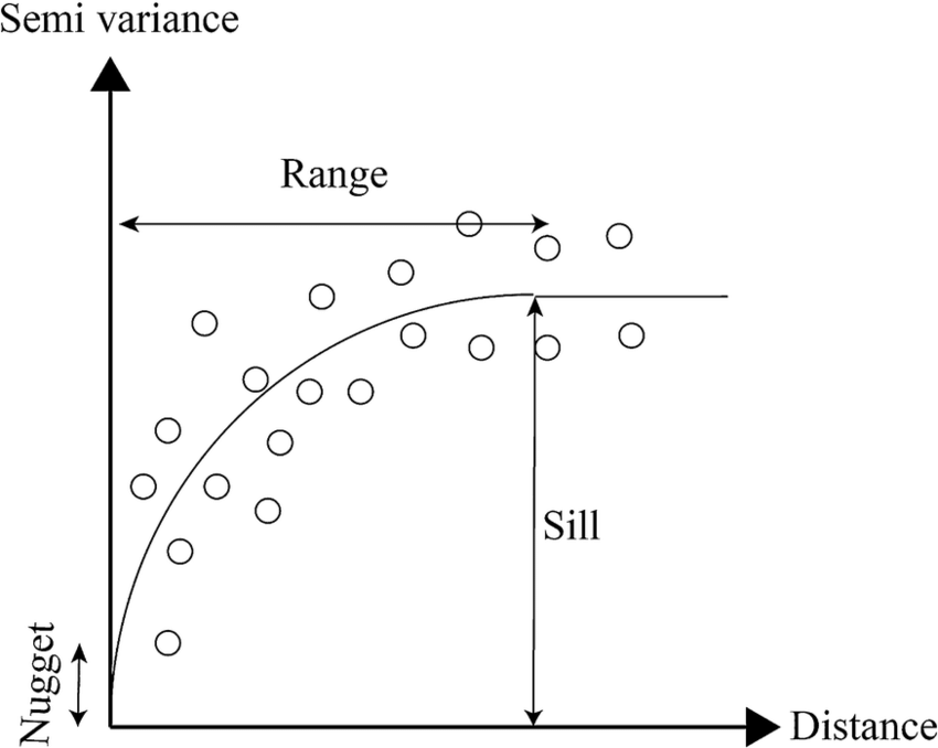
This diagram illustrates a typical semivariogram used in geostatistics, plotting semivariance against distance to understand spatial relationships in data. The 'nugget' represents variation at zero distance, the 'sill' shows where values level off, indicating maximum variance, and the 'range' is the distance where points become uncorrelated. Together, these elements guide the Kriging process for making spatial predictions (Ilias et al., 2015)

Kriging Estimator

The Kriging estimator for an unknown value at location x0 is given by a linear combination of known values:

\(z(x_0) = \sum_{i=1}^{N} \lambda_i z(x_i) \)

where:

z^(x0)z^(x0) is the estimated value at location x0x0,
z(xi)z(xi) are the known values at surrounding locations,
λiλi are the weights assigned to each known value, calculated to ensure unbiasedness and minimum variance of the estimator.

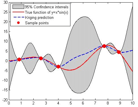
This graph showcases a Kriging model's prediction (red line) against the actual data trend (blue dashed line), with the shaded area representing the prediction uncertainty. It's a visual representation of how close the Kriging estimates are to the true values and the potential variance around those estimates (Suprayitno et al., 2018)

Objective of Kriging

The objective of Kriging is to minimize the variance of the estimation error, which leads to the Kriging variance.

Exactly, choosing a window size smaller than the sill for spatial data analysis, such as

Preparing Data for Analysis

Before we can perform Kriging, a method of interpolation for estimating unknown values across a geographic space, our data must be optimally prepared. This involves converting data into an efficient format, sampling, and determining clustering, which is facilitated by the script introduced previously.

As we discussed in a previous article, Kriging is a nonlinear process that does not lend itself to parallelization. The hack here is to break our spatial LiDAR scene into chunks, Krige each chunk individually on a separate thread in parallel, before finally combining the chunks and smoothing out edge artifacts.

Supporting LAS and LAZ Formats for Enhanced Workflow Robustness

Accepting LAS and LAZ file formats ensures the robustness of the geospatial data processing workflow. LAS, the standard format for storing LiDAR point cloud data, is widely used for its accessibility and ease of use; however, LAZ, the compressed version of LAS, offers significant advantages in terms of storage efficiency and transfer speed, which is particularly beneficial for handling large datasets and optimizing cloud storage costs. By accommodating both formats, workflows become more flexible and inclusive, allowing users to work with data in their preferred format without time-consuming conversions. This dual-format support ensures that processing pipelines can handle a broader range of datasets, enhancing the robustness and scalability of geospatial analysis projects.

Preparing to Read LAZ Files with Pylas

Before working with LAZ files in Python using Pylas, it's crucial to ensure that the LASzip decompression tool is available on your system since Pylas relies on it to read LAZ files. Here's how to set it up:

Download LASzip: Visit the LASzip website or the GitHub repository to download the LASzip executable or source code suitable for your operating system.

Install LASzip:

For executables, run the installer and follow the installation instructions.

If you're working from a source, compile LASzip according to the instructions provided in the repository.

Add LASzip to System Path:

Windows: Add the folder containing the LASzip executable to your system's PATH environment variable. This can be done from the System Properties > Advanced > Environment Variables dialog.

export PATH=$PATH:/path/to/laszip

Replace /path/to/laszip with the actual path where LASzip is installed.

Uploading LAZ Files to a Cloud Bucket

Once your LAZ files are ready and you can ensure Pylas can read them, uploading to a cloud storage bucket for processing or backup is straightforward. Here's a general approach using Google Cloud Storage (GCS) as an example:

Install Google Cloud SDK: If you haven't already, install the Google Cloud SDK from the official website.

Authenticate Your Session: Use the following command to authenticate with GCP:

gcloud auth login

Create a Cloud Storage Bucket: If you don't already have a bucket, create one using:

gsutil mb gs://your-bucket-name/

Replace your-bucket-name with a unique name for your bucket.

Upload LAZ File: Upload your LAZ file to the bucket using the gsutil cp command:

gsutil cp your-file.laz gs://your-bucket-name/path/to/target/

Replace your-file.laz with the path to your LAZ file and adjust the bucket path as needed.

This setup ensures that your LAZ files are backed up in the cloud and ready for further processing or analysis using cloud-based tools and services.

Thank you for reading TechTerrain: Innovations in Geospatial and Machine Learning. This post is public so feel free to share it.

Converting LAS/LAZ to Parquet

The script starts by converting LAS/LAZ files to Parquet format. Parquet is a columnar storage format that offers efficient data compression and encoding, essential for handling large geospatial datasets in distributed computing environments.

def convert_las_to_parquet(input_las_path, output_parquet_path):
    # Read the LAS/LAZ file
    las = pylas.read(input_las_path)

    # Convert LAS data to a pandas DataFrame
    # Extracting relevant fields, add or remove fields as needed
    data = {
        'x': las.x,
        'y': las.y,
        'z': las.z,
        'intensity': las.intensity,
        'classification': las.classification,
        'return_number': las.return_number,
        'number_of_returns': las.number_of_returns,
        # Add any other LAS attributes you need
    }
    df = pd.DataFrame(data)

    # Write the DataFrame to a Parquet file
    df.to_parquet(output_parquet_path, index=False)

    print(f"Converted {input_las_path} to {output_parquet_path}")

Why Optimal Window Sizes Matter

For effective Kriging, choosing an appropriate window size for analysis is essential. The window size determines the spatial extent to which we interpolate values from known points. By setting our window size to twice the sill, we ensure that our analysis window encompasses the area within which points are spatially correlated, maximizing the accuracy of our interpolated values.

The windowing strategy in Kriging, particularly for large datasets, is crucial due to the computational intensity of matrix inversions required for spatial interpolation, which scales cubically with the dataset size O(n^3). This makes processing large datasets computationally demanding and time-consuming.

We can significantly reduce the computational load by segmenting the data into smaller windows. Each window contains a manageable subset of points, ensuring the matrix inversion is feasible on a smaller scale. This enhances processing efficiency without compromising the accuracy of the interpolation.

Moreover, this approach allows for parallel processing. Each window can be assigned to a separate thread, enabling simultaneous computations. This not only speeds up the analysis but also optimizes resource utilization, making Kriging more practical and efficient for large spatial datasets.

Publishing Results and Next Steps

The script also includes functionality for publishing the analysis results to a Google Cloud Pub/Sub topic, enabling further processing or visualization in downstream applications. This step is crucial for integrating our geospatial analysis into larger data pipelines or systems.

def analyze_and_publish_pointcloud(parquet_file_path, x_mesh, y_mesh, project_id, topic_id):
    # Initialize Pub/Sub publisher
    publisher = pubsub_v1.PublisherClient()
    topic_path = publisher.topic_path(os.environ("PROJECT_ID"), os.environ("TOPIC_ID"))

    # Load the point cloud data from a Parquet file
    pointcloud_df = pq.read_table(parquet_file_path).to_pandas()

    # Sample data if necessary
    sampled_df = pointcloud_df.sample(n=min(1000, len(pointcloud_df)), random_state=0)

    # Determine the optimal number of clusters
    k_range = range(1, 11)
    sse = elbow_method(sampled_df[['x', 'y']], k_range)
    optimal_k = find_optimal_clusters(sse, k_range)
    print(f"Optimal number of clusters: {optimal_k}")

    # Stratify Sample Spatially using KMeans
    kmeans = KMeans(n_clusters=optimal_k, random_state=0).fit(sampled_df[['x', 'y']])
    indices = [np.where(kmeans.labels_ == i)[0][0] for i in range(optimal_k)]

    # Select representative points
    sampled_points = pointcloud_df.iloc[indices]

    # Calculate Semivariogram for the sample
    coordinates = sampled_points[['x', 'y']].values
    values = sampled_points['z'].values
    V = Variogram(coordinates, values, model='spherical', normalize=False)
    sill = V.describe()['sill']

    # Define window and buffer size based on sill
    window_size = sill * 2
    buffer_size = window_size * 0.1

    # Prepare message with results
    message = {
        "window_size": window_size,
        "buffer_size": buffer_size,
        "total_windows": optimal_k,  # Use optimal_k for the number of clusters/windows
        "sill": sill
    }

    # Serialize message for publishing
    message_data = json.dumps(message).encode("utf-8")

    # Publish results to Pub/Sub
    future = publisher.publish(topic_path, message_data)
    future.result()  # Ensure the publish completes
    print(f"Published analysis results to {topic_path}")

Conclusion and What's Next

This article has introduced the initial steps and concepts necessary for preparing geospatial data for advanced analysis with GCP's Dataproc service and Geospark. Understanding the process of converting data formats, determining optimal sampling and clustering, and the significance of semivariogram analysis is foundational for geospatial data science.

In the next part of our series, we will delve into the setup and execution of Kriging on a Dataproc cluster leveraging Geospark exploring how distributed computing power can be harnessed to perform geospatial interpolation at scale. Stay tuned to learn how to apply these concepts to efficiently uncover insights from your geospatial data.

Thank you for reading, and I hope you have learned something. If you like this content, please like, share, comment, and subscribe!

References:

Ilias, Grinias & Atzemoglou, Artemios & Kotzinos, Dimitris. (2015). Design and Development of an OGC Web Processing Service as a Framework for Applying Ordinary Kriging in Groundwater Management. Chorografies (Χωρο-γραφίες). 4. http://geo.teicm.gr/ojs/index.php/Chorografies/article/view/40.

Suprayitno, Suprayitno & Yang, Cheng-yu & Yu, Jyh-Cheng & Lin, Bor-Tsuen. (2018). Optimum Design of Microridge Deep Drawing Punch Using Regional Kriging Assisted Fuzzy Multiobjective Evolutionary Algorithm. IEEE Access. 6. 63905-63914. 10.1109/ACCESS.2018.2878047.

TechTerrain: Innovations in Geospatial and Machine Learning