Optimizing Geospatial Analytics: Strategic Sampling and Automation for Efficient LiDAR Data Processing


In the field of geospatial analytics, the challenge of extracting meaningful insights from raw data hinges on advanced computational techniques and the strength of the infrastructure that supports them. A prime example of this is seen in optimizing Kriging within the Google Cloud Platform using Dataproc and distributed computing. Kriging, a cornerstone method in geostatistics for interpolating unknown values across a geographical area based on known data points, is essential in processing LiDAR data to produce detailed terrestrial maps.
However, this process encounters significant hurdles when dealing with the vast amounts of data points generated by LiDAR technology. The creation of a global semivariogram, crucial for the Kriging method, becomes exceedingly complex and costly due to the prohibitive number of data points. Such a challenge necessitates a shift towards more inventive and practical solutions to manage the computational demands without sacrificing the quality and accuracy of the analysis.
In this context, a strategic approach to sampling emerges as a critical solution. Through selective data sampling, it's possible to efficiently navigate through the extensive datasets, choosing data points that accurately represent the larger dataset's spatial relationships. This article intends to explore the proposed methodology for effective sampling, aiming to balance computational efficiency with the precision of geospatial analysis. This discussion is designed to be accessible to readers across various levels of expertise, providing insights into the innovative strategies that are making significant contributions to advancements in geospatial data analysis.
Nugget: The nugget effect represents the semivariogram's value at the origin, which is the y-intercept of the curve. It signifies the minimum level of variance observed in the dataset, accounting for measurement errors or spatial variation at distances smaller than the smallest sampled interval. A high nugget value suggests a large amount of unexplained variability at very short distances, possibly due to measurement errors or microscale variations.
Sill: The sill is the plateau reached by the semivariogram, beyond which the variance between points does not increase with distance. It represents the total variance observed in the dataset. The difference between the sill and the nugget (sill minus nugget) reflects the spatially structured variance, which is the portion of variance that can be explained by the spatial configuration of the samples.
Range: The range is the distance at which the semivariogram first flattens out, reaching the sill. It indicates the extent of spatial correlation; within this distance, data points are considered to be spatially correlated to one another. Beyond the range, points are essentially uncorrelated, implying that the knowledge of a value at one location does not provide any information about values at locations beyond the range.
What are "Lags"?
In geostatistics, a "lag" refers to the distance between pairs of points in the spatial dataset. Lags are used to measure how much (or how little) pairs of points vary from one another as you move across the landscape. This variation is crucial for understanding spatial correlation—the degree to which one point's value can predict another's based on their relative distance.
Computing a Global Semivariogram: Step-by-Step
The process of computing a global semivariogram involves several key steps, each contributing to the final model that describes how spatial variance changes with distance across the entire study area. Here’s how it's typically done:
Define the Maximum Distance and Lag Size: First, determine the maximum distance across which to calculate spatial relationships. This distance should be large enough to encompass the spatial scope of your study area. Next, divide this distance into intervals or "lags" of equal size. The size of these lags can influence the resolution of your semivariogram.
Calculate Pairwise Distances: Compute the distance between every pair of sampled points in your dataset. This is where the O(n2) computational complexity comes into play, especially for large datasets.
Group Pairs by Lag: Assign each pair of points to a lag based on their calculated distance. This step organizes the data for variance calculation.
Calculate Semivariance for Each Lag: For each lag, calculate the semivariance—a measure of the variability between pairs of points within that lag distance. The formula for semivariance is:

γ(h) is the semivariance for the lag ℎh.
N(h) is the number of point pairs separated by lag distance ℎ.
Z(xi) is the value (such as arsenic concentration) at location xi.
Z(xi+h) is the value at a location a lag distance ℎh away from xi.
Plot the Semivariogram: Plot the calculated semivariance values against their corresponding lag distances. This plot reveals the spatial structure of the dataset, typically showing how semivariance increases with distance up to a certain point (the range) before leveling off (the sill).
Model Fitting: Finally, fit a theoretical model to the plotted semivariogram. This model, which could be spherical, exponential, or Gaussian, among others, mathematically describes the spatial correlation observed in your data. It's used in Kriging to make predictions at unsampled locations.
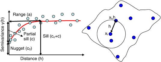
This diagram illustrates the components of a semivariogram and their relationship to spatial data points. On the left, the semivariogram graph displays the nugget (c₀), which represents measurement error or microscale spatial variation, the sill (c₀+c) which is the total variance, and the range (a) where spatial correlation is present. On the right, spatial points are shown with lags (h) indicating the distance between them, used to calculate semivariance for the semivariogram (Rama et. al., 2013)
Real World Example With ArcGIS
When I embarked on my first GIS class back in 2012, utilizing ArcGIS, I was introduced to the world of geospatial analysis through a project that hit close to home: estimating arsenic groundwater values in San Antonio. The task illuminated the complexities of environmental studies, especially when working with limited datasets. The challenge was not just about understanding the spread of arsenic—a notorious contaminant affecting water quality—but about doing so efficiently, with a sparse set of samples.
Note this is not the direct result from my lab, but this figure effectively illustrates the main concepts. The concentration map above is a raster image with each pixel containing an estimate of arsenic concentrations at that spatial location. This map can be georeferenced
In this context, the computation of all pairwise distances or "lags" between sampled points became a pivotal exercise. Given the O(n2) computational complexity, where n is the number of sampled points, our small dataset transformed what could have been a computational behemoth into a manageable task. This efficiency was crucial, allowing us to construct semivariograms swiftly and dive into Kriging analysis with a pace that larger datasets would not permit.
The end result was a detailed raster “heat-map” that could be overlaid atop aerial imagery of the city show concentrations at each spatial pixel.
Kriging LiDAR Point Cloud Data To Create Digital Elevation Models (DEMs)
When discussing the utilization of Light Detection and Ranging (LiDAR) technology in geospatial analysis, we're often faced with an overwhelming abundance of data. LiDAR systems collect millions of points that create detailed three-dimensional representations of the surveyed environment. While this data richness is invaluable for precision mapping and various analyses, it poses a significant computational challenge when performing geostatistical processes such as semivariogram calculations for Kriging interpolation.
The crux of the issue lies in the computation of lags—the measure of spatial correlation between pairs of points, which is central to developing the semivariogram. Ideally, a lag is calculated between every pair of points in the LiDAR dataset to understand the spatial structure fully. However, this process scales poorly with large datasets. Given the O(n2) computational complexity, where n is the number of points, the time required to compute a lag between each pair of points becomes prohibitively long, even after downsampling the dataset. Downsampling is a common strategy to reduce data volume, but it can only go so far before losing crucial detail, and even then, the remaining dataset may still be too large for exhaustive pairwise lag calculations.
For instance, let's consider a downsized LiDAR dataset where we've reduced the point cloud to a tenth of its original size. While this is a significant reduction, the computational load remains substantial. If we were to have 100,000 points post-downsampling—a modest number by LiDAR standards—the calculation would still involve computing the lags for 5 billion point pairs. The computational demands in terms of processing power and time are enormous, often exceeding the available resources or the project's time constraints.
This limitation is not just a technical problem; it has practical implications. In environmental monitoring, urban planning, or natural resource management, the timeliness of data processing can be crucial. Delays in generating the semivariogram can hinder timely decision-making, potentially leading to adverse outcomes in both project management and policy implementation.
In addressing the LiDAR challenge, we must recognize the need for a more efficient strategy to approximate the semivariogram for large datasets. Such a strategy would need to balance the detail captured by the point cloud with the practicality of computation, ensuring that the spatial analysis remains both feasible and informative. The development and application of innovative approaches that can handle the volume and complexity of LiDAR data efficiently are not just beneficial but necessary for advancing the field of geospatial analysis.
Need For Strategic Sampling
The efficient analysis of LiDAR data, especially within cloud computing environments like Google Cloud Platform, requires smart sampling strategies that can capitalize on the inherent spatial structure of the data. To inform our sampling approach, we first turn to Moran's I, a measure of spatial autocorrelation.
Understanding Moran's I
Moran's I is a statistic used to measure the degree of spatial autocorrelation in a dataset, ranging from -1 (indicating perfect dispersion) to +1 (indicating perfect correlation), with 0 representing random spatial patterns. A positive Moran's I suggests that similar values are clustered together in space, whereas a negative Moran's I indicates that similar values are dispersed and occur among dissimilar neighbors (Moran, 1950)
Strategic Sampling Based on Moran's I
Highly Positive Moran's I (Clustered Data): When Moran's I is significantly positive, it indicates a strong spatial correlation where points close to each other are likely to have similar values (Tsai et al., 2006). In this case, we employ cluster sampling. This technique involves dividing the study area into clusters that are likely to be internally homogeneous, and then randomly selecting a number of these clusters for analysis. By doing so, we ensure that our sample captures the essence of the spatial structure without the need to analyze every point. To ensure robustness, we can also choose a representative point from each cluster and calculate lags in between clusters as well.
Highly Negative Moran's I (Dispersed Data): Conversely, a highly negative Moran's I suggests that points with similar values are scattered throughout the space, indicating a pattern of spatial dispersion (Tsai et al., 2006). Systematic sampling becomes an appropriate strategy here. We would spread our sampling effort evenly across the entire study area to ensure that we capture the variability inherent in the data. This might involve creating a grid overlay across the study area and sampling at regular intervals, ensuring comprehensive coverage.
Moran's I Close to Zero (Random Distribution): When Moran's I is near zero, it implies no discernible spatial autocorrelation (Tsai et al., 2006). In such scenarios, the assumptions of the Central Limit Theorem (CLT) come into play, and we can take a simple random sample. The randomness of the sampling approach aligns with the lack of spatial structure, allowing for a fair representation of the entire dataset without bias towards any specific pattern of data distribution.
Automation in Cloud Computing
When sampling we cannot simply take a random sample as dictated by The Central Limit Theorem (CLT). The CLT assumes that sample observations are independent, an assumption which does not hold for LiDAR data due to spatial autocorrelation—nearby points are likely to have similar values. Since the CLT's premise is violated by the inherent nature of spatial data, it cannot be reliably applied to LiDAR datasets. Furthermore, the 'large enough' sample size required by the CLT is often beyond practical reach for high-resolution data like LiDAR, rendering the theorem unsuitable for simplifying the computational complexity of spatial analysis in this context.
Implementing these sampling strategies in a cloud computing environment can greatly benefit from automation. Cloud computing platforms can efficiently handle the intensive computations needed to calculate Moran's I for large datasets. Once the degree of spatial autocorrelation is understood, an automated sampling process can be triggered:
For clustered data, the system can automatically identify and select representative clusters.
For dispersed data, it can systematically apply a sampling grid and select points at regular intervals.
For random distributions, it can randomly generate sample points across the entire study area.
This automation not only speeds up the preliminary analysis but also ensures that the subsequent steps are tailored to the data's spatial characteristics, leading to more accurate and reliable interpretations from the LiDAR datasets. This strategic approach facilitates the handling of vast amounts of geospatial data, enabling detailed environmental analyses and insights without the prohibitive computational costs of exhaustive data processing.
Thank you for reading and I hope you’ve learned something. If you like this content, please like, share, comment, and subscribe to help the blog keep going!
Acknowledgements
I would like to extend my heartfelt gratitude to Robert Paradez for providing his expertise in statistical consulting for this blog post. His assistance was invaluable in shaping the content. Robert serves as a Statistics teacher at Cypress-Fairbanks ISD and also Statistics Lecturer at Lone Star College-CyFair Campus. He earned his Master of Science in Quantum Mechanics from the University Of Houston.

References
Cressie, N. (1993). "Statistics for Spatial Data". Wiley-Interscience. This book is a comprehensive source on spatial statistics, covering a wide range of topics including Kriging and its theoretical underpinnings.
Moran, P.A.P. (1950). "Notes on Continuous Stochastic Phenomena". Biometrika. 37 (1/2): 17–23. This is the seminal paper where Patrick Moran introduced the Moran's I statistic, a cornerstone in the field of spatial statistics.
Polizzotto, Matthew & Kocar, Benjamin & Benner, Shawn & Sampson, Michael & Fendorf, Scott. (2008). Near-Surface Wetland Sediments as a Source of Arsenic Release to Ground Water in Asia. Nature. 454. 505-8. 10.1038/nature07093.
Rama Mohan Pokhrel, Jiro Kuwano, Shinya Tachibana (2013)(, A kriging method of interpolation used to map liquefaction potential over alluvial ground, Engineering Geology, Volume 152, Issue 1,2013, Pages 26-37, ISSN 0013-7952, https://doi.org/10.1016/j.enggeo.2012.10.003.
Tsai, P.-J., Lin, M.-L., Chu, C.-M., & Perng, C.-H., published in "BMC Public Health" in 2009, is a notable example of applying Moran's I statistic in the field of public health to identify healthcare hotspots in Taiwan for the year 2006.
About the Author
Daniel Rusinek is an expert in LiDAR, geospatial, GPS, and GIS technologies, specializing in driving actionable insights for businesses. With a Master's degree in Geophysics obtained in 2020 from the University of Houston, Daniel has a proven track record of creating data products for Google and Class I rails, optimizing operations, and driving innovation. He has also contributed to projects with the Earth Science Division of NASA's Goddard Space Flight Center. Passionate about advancing geospatial technology, Daniel actively engages in research to push the boundaries of LiDAR, GPS, and GIS applications.