
Optimizing LiDAR Data Processing with Octree Downsampling on DataProc
A Comprehensive Guide to Efficient 3D Spatial Analysis

What is a Point Cloud?
Imagine taking a complex object or area and capturing every tiny detail about its surface by plotting millions of tiny dots (or points) in a 3D space. This collection of dots is what we call a point cloud. Each point represents a detailed piece of information about the object's or area's surface. First order of business is to down sample our LiDAR data.

Why Downsample?
While having a lot of detail is good, sometimes it's too much for computers to handle efficiently, especially if we need to process or analyze this data quickly. Downsampling is a way to simplify this data by reducing the number of points, making it easier and faster for computers to work with, without losing too much important information.
Moreover, downsampling in this way ensures that we maintain our data’s spatial integrity as much as possible.
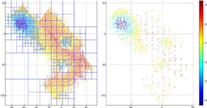
This figure showcases the effectiveness of an octree downsampling method, which streamlines a dense collection of data points by selectively thinning them out. The method ensures essential spatial relationships are retained, striking a balance between detail and computational efficiency (Zandara et al., 2013)
The Octree Downsampling Method
What is an Octree?
An octree is a way of dividing 3D space into smaller, manageable parts. Imagine a cube that represents the entire space of our point cloud. This cube is then divided into eight smaller cubes, or "octants." If any of these smaller cubes still has too many points (more than we've decided is manageable), we can divide it again into even smaller cubes. We keep doing this until all the cubes have a manageable number of points.
Downsampling with an Octree: Step-by-Step
Step 1: Create the Octree Structure
We start by creating our initial cube (the entire space of the point cloud) and then dividing it into smaller cubes based on how dense (how many points) different areas are.
Step 2: Divide Until Satisfactory
We continue to divide each cube into smaller cubes if they exceed our set limit of points. This process creates many smaller regions of space, each with a manageable number of points.
Step 3: Select Representative Points
For each of the smallest cubes, we now select a representative point. This could be the average position of all points in the cube or a randomly selected point. This step significantly reduces the number of points in our point cloud.
Step 4: Reconstruct the Simplified Point Cloud
Using all the representative points from the smallest cubes, we reconstruct the point cloud. This new point cloud has far fewer points, making it easier to handle.
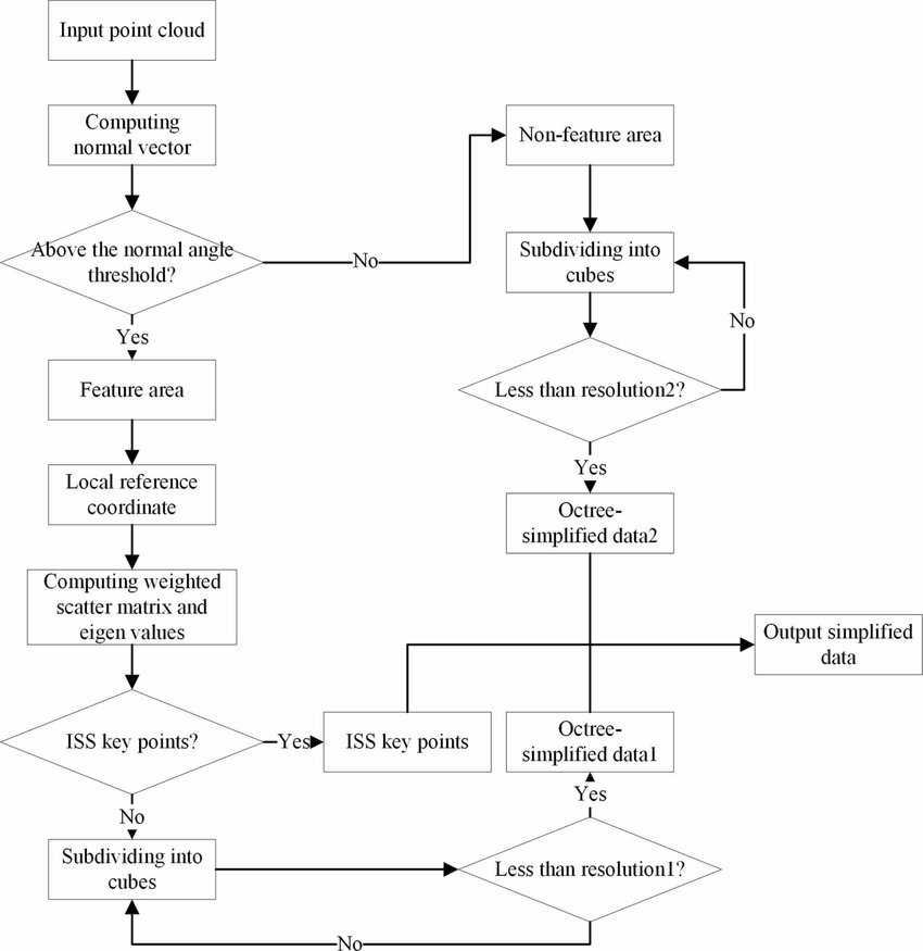
This flowchart delineates the LiDAR point cloud downsampling methodology, showcasing the critical step of identifying ISS key points—selective nodes based on geometric uniqueness in the data. Such nodes are instrumental in preserving the structural integrity of the point cloud during the simplification process, ensuring vital features are maintained even as data volume is reduced for efficiency (He et al., 2023).
Benefits of Using an Octree for Downsampling
The method is very efficient for large datasets.
It preserves the overall structure of the point cloud by ensuring that the simplification happens uniformly across the entire space.
It allows for varying levels of detail in different areas of the point cloud, depending on the complexity of the area.
Octeee Maintain Spatial Integrity
Spatial Integrity refers to the accuracy and consistency of the spatial arrangement and relationships between points in a point cloud. It's vital for ensuring that the simplified dataset still accurately represents the shape, structure, and distribution of the original object or area.
Why It Matters
Maintaining spatial integrity is crucial for any subsequent analyses or applications using the point cloud. Whether for constructing 3D models, performing measurements, or conducting spatial analyses, the reliability of the results depends heavily on the fidelity of the point cloud to the real-world objects or areas it represents.
import os
from google.cloud import storage
from pdal import Pipeline
import json

# Initialize Google Cloud Storage  client
client = storage.Client()
bucket_name = 'lidar-bucket'
bucket = client.get_bucket(bucket_name)

# Specify the LAS file to download
las_file_name = 'my-LiDAR-file.las'
local_las_path = f'/tmp/{las_file_name}'

# Download LAS file from GCS
blob = bucket.blob(las_file_name)
blob.download_to_filename(local_las_path)
print(f"Downloaded {las_file_name} to {local_las_path}")

# Define PDAL pipeline for octree downsampling
pipeline_definition = {
    "pipeline": [
        {
            "type": "readers.las",
            "filename": local_las_path
        },
        {
            "type": "filters.sample",
            "radius": "1.0"  # Adjust the radius based on your downsampling requirements
        },
        {
            "type": "writers.las",
            "filename": "/tmp/downsampled_output.las"
        }
    ]
}

pipeline_json = json.dumps(pipeline_definition)
pipeline = Pipeline(pipeline_json)

# Execute PDAL pipeline
pipeline.execute()
print("Downsampling completed. Output saved to /tmp/downsampled_output.las")

# At this point, you could upload the downsampled file back to GCS or continue processing
now we will convert this data into an RDD for distributed processing in GeoSpark.
from pyspark import SparkContext
from geospark.register import GeoSparkRegistrator

# Assuming 'data' is your list of dictionaries with 'X', 'Y', 'Z' coordinates
# and is already available in your current context.

# Initialize Spark Context
sc = SparkContext.getOrCreate()

# Register GeoSpark functions and types
GeoSparkRegistrator.registerAll(sc)

# Create an RDD from the existing data list
rdd = sc.parallelize(data)

# Now transform this RDD to include the Z value
# Here, we are simply keeping the Z value as part of a tuple (X, Y, Z)
spatial_rdd_with_z = rdd.map(lambda point: (point['X'], point['Y'], point['Z']))

# Your RDD now contains tuples with X, Y, and Z values that can
The next step is to find the nearest neighbors for each point on our digital terrain model—a kind of 3D map. In other words we pretend a point exists at the center each pixel in our blank initialized height map, and then find neighbors of that point to predict what its value should be. We'll use GeoSpark for this task. Once we've found the nearest points and how far away they are, we'll use a tool called a Semivariogram to figure out how much weight, or importance, each neighbor has.
So, what's a Semivariogram? It's a way of looking at the distance between every pair of points. Since there are so many pairs, this could take a very long time. To speed things up, we'll work with just a sample of all the points.
Sampling Assumptions
Here’s the tricky part: the locations on our map are not just scattered randomly; they are related to each other. Because of this, we can't just pick a random sample. Doing that would ignore the fact that what happens at one point on the map can affect what happens at another point. This kind of relationship means that our data doesn't follow the rules of the Central Limit Theorem, which expects that a large enough sample of random points will spread out in a predictable pattern. So, we need to be careful and select a sample that truly represents how points are related across the map, preserving the natural patterns of the terrain.
The methods for this ampling are a bit out of the scope of this post; we may come back to that in a future post. For now though, just keep the underlying principle in mind.
There too many LiDAR point pairs so we need to choose a sample, but cannot assume a random sample will represent the spatial relationships!
Finishing Up Our Gridding Process
Okay so back to gridding. For each grid cell we want to conduct a search query to find its neighbors within a search radius and apply weights to those based on our calculated semivariogram model. We will leverage our spatial partitioning here. See this article for more details:
The key point is that while Spark tells us which points are neighbors, it doesn't give us the distances between them. Luckily, since we have the XYZ coordinates, calculating the distance is straightforward. However, for large areas, using straight-line (Euclidean) distances isn’t accurate because the Earth is round. For small areas, it's fine to use Euclidean distances, but for larger spaces, we should use the haversine formula or calculate great circle distances instead.
from pyspark import SparkContext, SparkConf
from geospark.register import GeoSparkRegistrator
from geospark.core.SpatialRDD import PointRDD, SpatialRDD
from geospark.core.geom.envelope import Envelope
from geospark.core.formatMapper.wkt_reader import WktReader
from shapely.geometry import Point, Polygon
import numpy as np

# Initialize Spark and GeoSpark
conf = SparkConf().setAppName("KrigingExample")
sc = SparkContext(conf=conf)
GeoSparkRegistrator.registerAll(sc)

# Assuming the bounding box of the LiDAR data is given as follows:
# minX, maxX, minY, maxY represent the spatial extent of the LiDAR data
  # Example values, replace with your actual data

# Desired spatial resolution (distance between points in the grid)
resolution = 10  # Example value, replace with your desired resolution

# Calculate the number of grid cells based on the spatial extent and resolution
#Can get spatial extent from LAS file.
x_range = np.arange(minX, maxX, resolution)
y_range = np.arange(minY, maxY, resolution)

# Generate grid cells
grid_cells = [(x, y) for x in x_range for y in y_range]

# Parallelize the grid cells into an RDD
grid_rdd = sc.parallelize(grid_cells)

# From here, you would proceed with the neighbor search, distance calculation, and Kriging

Function to integrate your semivariogram for weight calculation
def calculate_weight_with_semivariogram(distance, semivariogram):
    # Here you would calculate the weight using your semivariogram model
    # This is a placeholder for the actual calculation
    # You might use a model like: weight = semivariogram(distance)
    weight = semivariogram(distance)
    return weight

# Modify the find_neighbors_and_distances function to use the semivariogram for weight calculations
def find_neighbors_and_distances_with_semivariogram(point, neighbors_rdd, radius, semivariogram_model):
    # Find neighbors within radius R
    neighbors = neighbors_rdd.filter(lambda x: point.distance(x) <= radius).collect()

    # Calculate distances and assign weights using the semivariogram model
    weighted_neighbors = []
    for neighbor in neighbors:
        distance = point.distance(neighbor)
        weight = calculate_weight_with_semivariogram(distance, semivariogram_model)  # Use the semivariogram model for weight
        weighted_neighbors.append((neighbor, weight))

    return weighted_neighbors

# Modify the assign_z_value_to_prediction_point function accordingly
def assign_z_value_to_prediction_point_with_semivariogram(x, y, point_rdd, R, semivariogram_model):
    prediction_point = Point(x, y)
    weighted_neighbors = find_neighbors_and_distances_with_semivariogram(prediction_point, point_rdd, R, semivariogram_model)

    # Compute weighted Z value using the weights from the semivariogram model
    weighted_sum = sum(neighbor[1] * neighbor[0].z for neighbor in weighted_neighbors)
    total_weights = sum(neighbor[1] for neighbor in weighted_neighbors)
    z_value = weighted_sum / total_weights if total_weights != 0 else 0

    return z_value

# Assuming you've initialized your Spark context and GeoSparkRegistrator as before

# Radius for neighbor search
R = 5

# Loop through the grid and assign Z values using the semivariogram model
z_values_rdd = grid_rdd.map(lambda cell: assign_z_value_to_prediction_point_with_semivariogram(cell[0], cell[1], point_rdd, R, my_semivariogram))

# This code now integrates your semivariogram model into the Kriging process, improving the accuracy of weight assignments based on spatial correlation.
Once we have the distances, we can assign weights to each point and figure out the elevation at our target location.
Thanks to GeoSpark, we can do a lot of this work in parallel, speeding things up. This is a big deal because traditional methods like Kriging, while accurate, are slow. See this previous post for more details!

Finally, we'll use Google Earth Engine to create a "tiled image" for Google Maps. This is a clever way to manage data so that when you zoom out, you see a lower resolution, and it gets sharper as you zoom in, but only for the part of the map you're looking at. We'll dive deeper into how we use Google Earth Engine and Mapbox later.
Thank you for reading and hope you’ve learned something. If you like this content please, like, comment, share and subscribe!
References
He, Leping & Yan, Zhongmin & Hu, Qijun & Xiang, Bo & Xu, Hongbiao & Bai, Yu. (2023). Rapid assessment of slope deformation in 3D point cloud considering feature-based simplification and deformed area extraction. Measurement Science and Technology. 34. 10.1088/1361-6501/acafff.
Zandara, Simone & Ridao, Pere & Romagós, David & Mallios, Angelos & Palomer, Albert. (2013). Probabilistic Surface Matching for Bathymetry Based SLAM. Proceedings - IEEE International Conference on Robotics and Automation. 10.1109/ICRA.2013.6630554.
About the Author
Daniel Rusinek is an expert in LiDAR, geospatial, GPS, and GIS technologies, specializing in driving actionable insights for businesses. With a Master's degree in Geophysics obtained in 2020 from the University of Houston, Daniel has a proven track record of creating data products for Google and Class I rails, optimizing operations, and driving innovation. He has also contributed to projects with the Earth Science Division of NASA's Goddard Space Flight Center. Passionate about advancing geospatial technology, Daniel actively engages in research to push the boundaries of LiDAR, GPS, and GIS applications.