Optimizing Geospatial Workflows in the Cloud: Continued
Harnessing the Power of Kubernetes, Apache Airflow, and Data Lakes for Advanced LiDAR Data Processing

Modernizing Geospatial Workflows with Cloud Technologies: Google Kubernetes Engine (GKE), Cloud Run, and More
The evolution of geospatial technologies towards cloud-based solutions marks a significant shift in the field of spatial data analysis. This transition addresses the need for scalable, accessible, and collaborative geospatial processing capabilities that traditional desktop-based tools struggle to provide. A notable challenge in this migration is adapting essential geospatial libraries, such as GDAL (Geospatial Data Abstraction Library), to the distributed and scalable nature of cloud environments.

This blog post is a continuation on discussions from this blog post:

there’s some more homework for you..
Overcoming GDAL Challenges in the Cloud
Here I will example a simplified Kubernetes and Apache Airflow architecture By leveraging the auto-scaling and container orchestration capabilities of Kubernetes, alongside the workflow management features of Apache Airflow, this approach ensures that geospatial data processing is both scalable and efficient.
Scalability: Kubernetes facilitates the dynamic allocation of resources, allowing GDAL-based operations to efficiently scale in response to varying workloads.
Data Access: Optimized access to cloud storage is achieved through Kubernetes volumes and Airflow's data staging mechanisms, ensuring that GDAL processes can efficiently read and write geospatial data.
Dependency Management: Containerization simplifies the deployment of GDAL, encapsulating its dependencies and ensuring consistent execution environments across development and production.
Argument: Embracing Data Lakes for Geospatial Excellence
In the domain of geospatial analysis, where the volume, variety, and complexity of data are ever-increasing, the strategic adoption of cloud storage, specifically data lakes, is imperative. LiDAR data, known for its voluminous unstructured nature, alongside associated GPS information and other metadata, finds an ideal storage solution in data lakes. This preference stems from several key characteristics of data lakes that align perfectly with the needs of geospatial data management and processing.
Improved Flexibility with Raw Data
Data lakes excel in storing raw data without the immediate need for structuring or preprocessing. This capability is particularly beneficial for geospatial datasets:
Direct Storage of Raw Data: Data lakes can store vast amounts of raw LiDAR point clouds and GPS data, preserving the original integrity and detail of the data. This raw storage capability ensures that data lakes can accommodate the diverse and dynamic nature of geospatial data without constraining it to a predefined schema.
Adaptive Analysis: The schema-on-read approach of data lakes allows for the flexible application of structure at the time of query or analysis. This adaptability is crucial for geospatial data, which benefits from tailored analytical processes that can evolve with project requirements.
Hypothetical Example
Imagine a tech firm called GeoEniroTech; they have an application that ingests client LiDAR data which has been uploaded to cloud storage, processes it on the cloud, and displays the results in a UI…
GeoEnviroTech could encounter a situation where both LAS 1.2 and LAS 1.3 datasets were uploaded by the client unknowingly; perhaps field crews used different LiDAR instruments when collecting data. While both versions share common XYZ coordinate data, LAS 1.3 files include additional attributes such as waveform data, which are not recognized by systems only configured for LAS 1.2 schema. This discrepancy poses a risk of causing errors or crashes in processing pipelines that are not designed to handle the variable schema.
Las 1.2 Header Block
Item                             | Format            | Size (bytes) | Required
--------------------------------------------------------------------------------
File Signature ("LASF")          | char[4]           | 4            | *
File Source ID                   | unsigned short    | 2            | *
Global Encoding                  | unsigned short    | 2            | *
Project ID - GUID data 1         | unsigned long     | 4            | *
Project ID - GUID data 2         | unsigned short    | 2            | *
Project ID - GUID data 3         | unsigned short    | 2            | *
Project ID - GUID data 4         | unsigned char[8]  | 8            | *
Version Major                    | unsigned char     | 1            | *
Version Minor                    | unsigned char     | 1            | *
System Identifier                | char[32]          | 32           | *
Generating Software              | char[32]          | 32           | *
File Creation Day of Year        | unsigned short    | 2            |
File Creation Year               | unsigned short    | 2            |
Header Size                      | unsigned short    | 2            | *
Offset to point data             | unsigned long     | 4            | *
Number of Variable Length Records| unsigned long     | 4            | *
Point Data Record Length         | unsigned short    | 2            | *
Number of point records          | unsigned long     | 4            | *
Number of points by return       | unsigned long[5]  | 20           | *
X scale factor                   | double            | 8            | *
Y scale factor                   | double            | 8            | *
Z scale factor                   | double            | 8            | *
X offset                         | double            | 8            | *
Y offset                         | double            | 8            | *
Z offset                         | double            | 8            | *
Max X                            | double            | 8            | *
Max Y                            | double            | 8            | *
Max Z                            | double            | 8            | *
Min X                            | double            | 8            | *
Min Y                            | double            | 8            | *
Min Z                            | double            | 8            | *
Las 1.4 Header Block
Item                                   | Format              | Size (bytes) | Required
-------------------------------------------------------------------------------------
File Signature ("LASF")                | char[4]             | 4            | yes
File Source ID                         | unsigned short      | 2            | yes
Global Encoding                        | unsigned short      | 2            | yes
Project ID - GUID Data 1               | unsigned long       | 4            | yes
Project ID - GUID Data 2               | unsigned short      | 2            | yes
Project ID - GUID Data 3               | unsigned short      | 2            | yes
Project ID - GUID Data 4               | unsigned char[8]    | 8            | yes
Version Major                          | unsigned char       | 1            | yes
Version Minor                          | unsigned char       | 1            | yes
System Identifier                      | char[32]            | 32           | yes
Generating Software                    | char[32]            | 32           | yes
File Creation Day of Year              | unsigned short      | 2            | yes
File Creation Year                     | unsigned short      | 2            | yes
Header Size                            | unsigned short      | 2            | yes
Offset to Point Data                   | unsigned long       | 4            | yes
Number of Variable Length Records      | unsigned long       | 4            | yes
Point Data Record Format               | unsigned char       | 1            | yes
Point Data Record Length               | unsigned short      | 2            | yes
Legacy Number of Point Records         | unsigned long       | 4            | yes
Legacy Number of Point by Return       | unsigned long[5]    | 20           | yes
X Scale Factor                         | double              | 8            | yes
Y Scale Factor                         | double              | 8            | yes
Z Scale Factor                         | double              | 8            | yes
X Offset                               | double              | 8            | yes
Y Offset                               | double              | 8            | yes
Z Offset                               | double              | 8            | yes
Max X                                  | double              | 8            | yes
Max Y                                  | double              | 8            | yes
Max Z                                  | double              | 8            | yes
Min X                                  | double              | 8            | yes
Min Y                                  | double              | 8            | yes
Min Z                                  | double              | 8            | yes
Start of Waveform Data Packet Record   | unsigned long long  | 8            | yes
Start of First Extended Variable Length Record | unsigned long long | 8    | yes
Number of Extended Variable Length Records      | unsigned long      | 4    | yes
Notice the difference in the schemas; specifically, LAS 1.4 includes waveform information! For more info on the differences see this article:

If an app user accidentally uploaded LAS 1.4 and, for example, Data Warehouse was expecting 1.2, the app could crash!
To address this challenge, GeoEnviroTech leverages the capabilities of data lake architecture, which excels in handling schema variability through schema-on-read and dynamic processing pipelines. When LAS files are ingested into the data lake, metadata extraction processes identify the LAS version of each file and tag it accordingly. This metadata is then utilized by GeoEnviroTech's processing pipelines, which are designed to dynamically adjust to the data's schema based on its version tag. For LAS 1.3 files, the pipeline includes conditional logic to process additional attributes, ensuring that these data are correctly handled and utilized without disrupting the overall workflow. Conversely, when processing LAS 1.2 files, the pipeline adapts to exclude steps related to non-existent attributes.
This approach ensures that GeoEnviroTech's analyses remain consistent and accurate, regardless of the LAS version. Furthermore, by storing raw data in the data lake and leveraging metadata-driven processing strategies, GeoEnviroTech maintains the flexibility to update their pipelines as new LAS versions are released or as project requirements evolve. This forward-thinking strategy not only mitigates the risk of processing errors but also positions GeoEnviroTech at the forefront of technological adaptability in environmental consulting.
This real-world-inspired example underscores the importance of flexible data management systems like data lakes in navigating the complexities of geospatial data analysis. By embracing such technologies, organizations can ensure the integrity and reliability of their data-driven insights, even in the face of evolving data formats and standards.
Integrated and Comprehensive Data Management
Data lakes serve as an integrated repository for all geospatial data types, facilitating complex analyses that leverage multiple data sources:
Unified Data Repository: By accepting raw LiDAR, GPS, and supplementary datasets in their native formats, data lakes eliminate the silos often encountered in traditional data storage. This consolidation enables more cohesive and comprehensive geospatial analyses.
Advanced Analytics and Machine Learning: The retention of raw data in data lakes not only supports traditional geospatial analyses but also empowers advanced analytics and machine learning. Researchers can access the full depth and breadth of the data, unleashing the potential for innovative insights and solutions.
The shift towards utilizing data lakes for geospatial data storage represents a strategic alignment with the modern demands of data volume, complexity, and analytical flexibility. For LiDAR and associated datasets, the choice of data lakes offers a scalable, adaptable, and comprehensive solution that traditional data warehouses and storage methods cannot match. In embracing data lakes, the geospatial community ensures that it can fully leverage the rich potential of its data, driving forward the boundaries of environmental understanding, urban planning, and beyond.
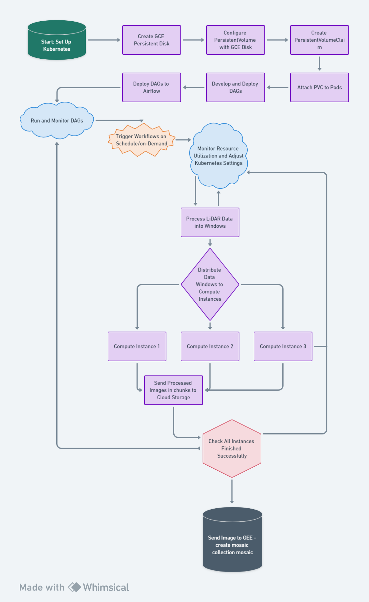
Now let’s set up Kubernetes:
1. Set Up Kubernetes
Kubernetes Cluster: The first step is to set up a Kubernetes cluster. This can be done on cloud platforms (like Google Kubernetes Engine on Google Cloud, Amazon EKS on AWS, or Azure Kubernetes Service on Azure) or on-premises using tools like Minikube or kubeadm, depending on your requirements and resources.
Persistent Storage: For geospatial applications, consider setting up persistent volumes in Kubernetes. Geospatial datasets can be large, and your workflows may require access to this data across various pods.
Networking and Security: Configure networking for inter-pod communication and define security policies as required for your application.
2. Install and Configure Apache Airflow in Kubernetes
Airflow on Kubernetes: You can run Apache Airflow within Kubernetes to leverage its powerful scheduling and workflow management capabilities. This can be achieved using the official Airflow Helm chart, which simplifies the deployment of Airflow on Kubernetes.
Helm Chart: Helm is a package manager for Kubernetes. The Airflow Helm chart will define all the necessary Kubernetes resources (Deployments, Services, Volumes, etc.) required to run Airflow. It allows for easy updates and management of the Airflow deployment.
Customize Airflow Configuration: Configure Airflow to meet your specific needs, such as executor types (e.g., CeleryExecutor, KubernetesExecutor) and Airflow DAGs directory. The KubernetesExecutor is particularly useful in dynamically allocating resources for each task as a separate pod, allowing for better resource management and scaling.
3. Develop and Deploy DAGs
DAG Development: Develop your Directed Acyclic Graphs (DAGs) to define the workflows. In the context of geospatial data processing, a DAG might include tasks for data ingestion, preprocessing, analysis (e.g., running geospatial algorithms), and post-processing (e.g., generating reports or visualizations).
DAG Deployment: Once developed, deploy your DAGs to Airflow. This typically involves placing your DAG code in a directory that Airflow scans for new DAGs, specified in the Airflow configuration.
4. Run and Monitor DAGs
Triggering Workflows: With Airflow running on Kubernetes, you can now trigger your DAGs either on a schedule or on-demand. Airflow provides a web interface to monitor and manage the execution of your workflows.
Scaling and Resource Management: Kubernetes, together with the KubernetesExecutor in Airflow, allows for dynamic scaling of resources per task. You can monitor resource utilization and adjust your Kubernetes cluster settings accordingly to optimize performance and cost.
The Necessity of a Stitching Approach for GDAL in Parallel Processing
When it comes to processing large geospatial datasets like LiDAR data, the use of GDAL (Geospatial Data Abstraction Library) is widespread due to its powerful capabilities in handling raster and vector data formats. However, GDAL's architecture presents certain limitations in parallel processing scenarios, which are increasingly common in the era of big data and cloud computing. This limitation underscores the necessity of adopting a stitching approach when leveraging GDAL for processing tasks that require scalability and efficiency.
GDAL's Parallel Processing Limitations
GDAL, while robust and versatile, is primarily designed for sequential processing. It excels in single-threaded operations but does not inherently support parallel processing of data. This design limitation becomes a bottleneck when dealing with vast datasets, such as those generated by LiDAR technology, where the ability to process data in parallel significantly reduces computation time and enhances efficiency.
Why a Stitching Approach is Essential
To circumvent GDAL's limitations in parallel processing and harness the power of cloud computing and modern multi-core processors, a stitching approach becomes crucial. This method involves:
1. Dividing the Dataset: Breaking down the large dataset into smaller, manageable tiles or chunks that can be processed independently. This division allows for the distribution of processing tasks across multiple cores or nodes.
2. Parallel Processing: Each chunk is processed simultaneously using separate GDAL instances. This step leverages the infrastructure's parallel processing capabilities, significantly speeding up the overall processing time.
3. Stitching Processed Chunks: After processing, the individual chunks are stitched or merged back together to form the complete dataset. This final step requires careful handling to ensure data continuity and integrity across the seams where chunks are joined.
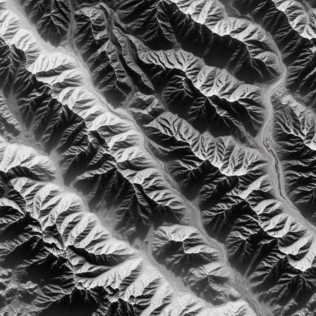
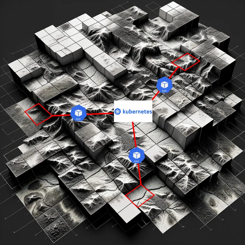
Our goal is to grid our LiDAR scene into a comprehensive Digital Elevation Model (DEM) (top image). To speed up processing we break this area into actual spatial blocks, and each block can now be processed separately but in a separate container or compute instance; the only caveat is that we need to stitch these back together in a way that avoids any data artifacts. Hence, we leverage Google Earth Engine (GEE) to do the stitching for us!
Advantages of the Stitching Approach
Scalability: By enabling parallel processing, the stitching approach allows GDAL-based workflows to scale with the available computing resources, making it suitable for cloud environments and large-scale data processing tasks.
Efficiency: Processing data in parallel dramatically reduces the time required to analyze and process large datasets, improving operational efficiency and enabling more timely insights.
Flexibility: This approach provides the flexibility to adjust the granularity of the processing tasks based on the computational resources available, optimizing the balance between processing speed and resource utilization.
Although GDAL's architecture presents challenges for parallel processing, adopting a stitching approach offers a viable solution to leverage GDAL effectively for large-scale geospatial data processing tasks. This method not only mitigates GDAL's limitations but also capitalizes on the advantages of distributed computing environments, ensuring that geospatial workflows can meet the demands of processing large datasets like those generated by LiDAR technology. By embracing this approach, organizations can enhance their geospatial processing capabilities, achieving greater scalability, efficiency, and flexibility in their operations.
As we advance into the next phase of our project, it's crucial to address how we'll tackle the gridding process for each LiDAR data window. Given the complexity and computational intensity of our geospatial workflows, particularly those involving extensive datasets from LiDAR technology, we must choose our orchestration and execution frameworks wisely. While Google Cloud Run offers notable advantages for certain application types, it falls short of meeting the specific demands of our project, which include intensive computational resources and advanced workflow orchestration. This is where Kubernetes and Apache Airflow come into play, providing a more apt solution for our needs.
Kubernetes: Custom-Fit for Our Compute-Heavy Workloads
Our geospatial workflows, especially the gridding process for each window, require significant computational power and flexibility in managing large datasets. Kubernetes stands out by offering an environment that's tailor-made for such compute-intensive tasks.
Resource-Intensive Operations: Diverging from Cloud Run's request-based scaling, Kubernetes introduces auto-scaling based on CPU and memory usage. This feature is indispensable for our project, accommodating the fluctuating computational demands of our geospatial processing tasks efficiently.
Stateful Workflows: Our project's nature necessitates maintaining state information throughout the processing steps. Kubernetes facilitates this through its support for persistent volumes and StatefulSets, ensuring our workflows remain cohesive and uninterrupted— a critical advantage over Cloud Run's stateless architecture.
Apache Airflow: Mastering Workflow Orchestration
To complement Kubernetes, Apache Airflow offers the sophisticated workflow orchestration needed to handle our project's complexity effectively.
Complex Dependency Management: Airflow's capability to define intricate task dependencies ensures that each step of our geospatial data processing, particularly the gridding of LiDAR windows, is executed in precise order and only when all necessary conditions are met. This level of dependency management is crucial for maintaining the integrity and efficiency of our workflows.
Dynamic Task Generation: The dynamic nature of our geospatial data, with its variable volume and characteristics, demands a workflow system that can adapt responsively. Airflow's support for dynamic task generation and parameterization allows our workflows to adjust seamlessly to the data being processed, ensuring optimal efficiency and accuracy.
In conclusion, while Cloud Run offers simplicity and efficiency for certain types of applications, it does not align with the specific requirements of our geospatial data processing project. The combination of Kubernetes and Apache Airflow, with their robust support for resource-intensive operations, stateful workflows, and complex workflow orchestration, presents a strategic solution that meets our project's demands. By adopting Kubernetes and Airflow, we're not just optimizing our resources for the task at hand; we're also ensuring the flexibility and control needed to navigate our complex, multi-stage processing workflows successfully. This strategic choice empowers us to fully harness the capabilities of modern cloud computing technologies, paving the way for innovative advancements in our geospatial data processing endeavors."
The complexity and scale of processing LiDAR data for creating a mosaic collection in Google Earth Engine (GEE) necessitate a coordinated, reliable, and efficient workflow management system. A Directed Acyclic Graph (DAG) in Apache Airflow provides the structured approach required to meet these challenges head-on. Implementing a DAG for this process is not just beneficial; it's imperative for several compelling reasons.
NOTE: If the spatial area to be processed is small, a Cloud Run instance might suffice. It is always important to understand the nuances of your data to make the most informed and cost-effective decision.
Sequential and Parallel Task Management
Structured Workflow: The process of transforming LiDAR data into a GEE mosaic collection involves multiple stages, including data preprocessing, windowing, processing each window, and finally, aggregation. A DAG organizes these tasks in a clear, logical sequence, ensuring that each step is completed in the correct order. This structured approach is crucial for maintaining the integrity and accuracy of the final mosaic.
Parallel Processing Efficiency:** Given the potentially vast number of windows derived from the LiDAR data, processing each one sequentially would be time-prohibitive. A DAG allows for the parallel processing of these windows, significantly accelerating the workflow. Airflow's DAGs manage these parallel tasks effectively, ensuring that resources are utilized optimally without compromising the workflow's overall cohesion.
Dependency and Error Handling
Complex Dependency Management: The creation of a GEE mosaic from LiDAR data involves tasks with complex dependencies. Some tasks cannot commence until others are completed, while some can proceed in parallel. A DAG explicitly defines these dependencies, ensuring that the workflow progresses smoothly without manual intervention.
Robust Error Handling: In any large-scale data processing task, errors are inevitable. A DAG in Airflow enables sophisticated error-handling mechanisms, including task retries, error notifications, and even skipping or branching based on error types. This robust error handling is crucial for minimizing disruptions in the workflow and ensuring that the process reaches completion.
Dynamic Scalability and Resource Optimization
Adaptive Task Scheduling: The workload in processing LiDAR data for a GEE mosaic can vary greatly depending on the data's volume and complexity. A DAG provides the flexibility to dynamically scale processing resources based on the workload, ensuring that each window is processed efficiently and cost-effectively.
Resource Allocation: By managing the task execution order and parallelism within a DAG, Airflow can optimize the allocation of computational resources. This prevents resource contention and ensures that each processing step has the resources it needs without wasting computational power on idle or unnecessary tasks.
Final Aggregation and Quality Assurance
Ensuring Complete Processing: The final step of creating a mosaic collection in GEE requires that all windows have been successfully processed and are ready for aggregation. The DAG approach guarantees that this aggregation only occurs after all dependencies are met, ensuring the completeness and integrity of the final product.
Quality Control: Incorporating quality control checks as part of the DAG allows for the automated verification of processed windows before their aggregation into the GEE mosaic. This step is crucial for ensuring that the final mosaic meets the project's quality standards.
Overall, implementing a DAG for processing LiDAR data into a GEE mosaic collection addresses the workflow's inherent complexity, scale, and need for reliability. The structured, flexible, and efficient nature of a DAG ensures that resources are optimized, errors are managed, and all processing steps are completed in the correct sequence. This approach not only maximizes efficiency but also ensures the high quality and integrity of the final mosaic collection, making it an indispensable strategy in the geospatial data processing workflow.
Networking Considerations Scenario: Advanced Geospatial Analysis on Demand
Imagine a feature in your application where users can perform advanced geospatial analysis directly from the interface where they view the DEM in Mapbox or Google Maps. For instance, a user might want to identify and analyze watershed areas within a selected region of the DEM or calculate slope gradients for land use planning. This type of analysis goes beyond static data visualization and requires on-the-fly processing of geospatial data based on user inputs.
Networking Consideration: Real-time Data Processing Requests
User Interaction:
The user selects a region on the DEM displayed in the front-end and requests a specific analysis, such as watershed delineation.
Sending Request to the Server:
This action triggers a network request from the client application to your backend server. Here, networking layers come into play, particularly:
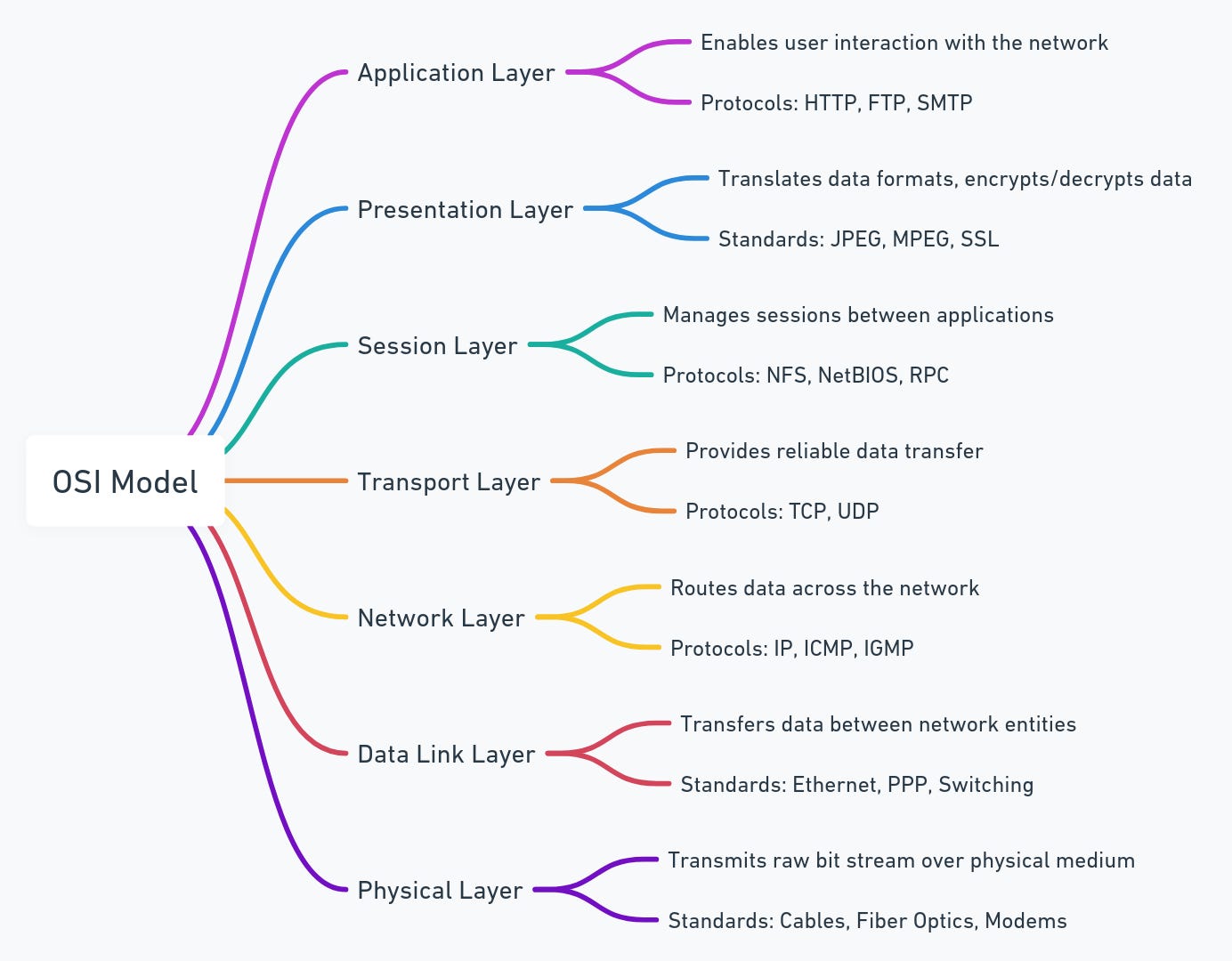
Layer 7 (Application Layer): HTTP/HTTPS protocols are used to format the request from the client.
Layer 4 (Transport Layer): Ensures reliable transmission of the request to the server, using TCP.
Layer 3 (Network Layer): IP protocols route the request to the correct server.
Server-side Processing:
The server receives the request and may need to interact with a cloud-based processing service (running in Kubernetes) to perform the requested analysis. This involves internal networking within the cloud environment to dispatch the job, manage data access from storage, and process the analysis.
Job Queuing and Execution:
Depending on the complexity, the server queues the processing job (using something like Apache Airflow) and executes it. The process might involve accessing additional geospatial data, running computational models, and generating new data layers.
Returning Results:
Once the analysis is complete, the results are sent back to the user through the network, involving the same layers in reverse order. The application layer (Layer 7) is particularly involved in formatting the response, which might include new data layers to be rendered on the map.
Dynamic Map Update:
The frontend application updates the DEM visualization with the analysis results, such as highlighting watershed areas or displaying slope gradients. This step might involve additional calls to Mapbox or Google Maps APIs, further engaging network protocols.
Here's an option to consider: Pub/Sub operates at the Application Layer (Layer 7) of the OSI model and serves as a robust messaging queue that facilitates asynchronous communication across different components of a cloud-based geospatial application. This service showcases how cloud platforms utilize the OSI framework to create architectures that are scalable, resilient, and decoupled. With Pub/Sub, handling large data workloads from sources like LiDAR or satellites becomes more efficient and faces less latency, allowing developers to concentrate on the application's logic instead of the complexities of lower networking layers. Incorporating the OSI model in the design and analysis of cloud services like this provides a clear understanding of the data flow—from initiating user interactions for geospatial computations to delivering the processed data, all organized within the structured network communication layers.
Networking Challenges and Considerations:
Latency and Performance: Real-time or near-real-time processing and visualization of geospatial data can be latency-sensitive. Optimizing network communication and processing efficiency becomes crucial.
Scalability: Handling multiple simultaneous user requests for data processing requires scalable backend infrastructure, which might involve auto-scaling Kubernetes deployments based on demand.
Security: Transmitting user requests and geospatial data analysis results necessitates robust security measures, including data encryption in transit (TLS/SSL) at the Transport Layer and authentication and authorization at the Application Layer.
This scenario illustrates how, even in applications primarily focused on data processing and visualization, networking layers and considerations become critically important when introducing dynamic, on-demand data analysis features that require server-side processing and real-time interaction with the user.
Kubernetes for Heavy, On-Demand Geospatial Processing
For applications expecting heavy and possibly unpredictable on-demand geospatial processing, Kubernetes (GKE) offers several advantages:
Vertical Pod Autoscaler (VPA): Kubernetes can automatically scale the memory and CPU resources to meet demand; great for processing LiDAR where each window could have different point densities, therefore variable LAS file sizes. VPA can anticipate a heavier workload on one pod and adjust resources accordingly.
Horizontal Pod Autoscaling (HPA): For more advanced geospatial analytics involving back-and-forth manipulation between the UI and backend, Kubernetes can add or remove pods as needed to meet demand
Resource Management: Kubernetes provides fine-grained control over CPU and memory allocations, allowing you to tailor resources to the specific needs of heavy processing tasks. This is crucial for optimizing performance and cost when dealing with complex geospatial analyses.
Stateful Workloads: If your geospatial processing tasks require maintaining state or involve complex transactions, Kubernetes supports stateful workloads with persistent storage options, offering more flexibility than stateless environments.
Cloud Run for Less Frequent LiDAR Processing
Cloud Run could be a more cost-effective and simpler solution for scenarios where LiDAR processing tasks are not performed frequently or predictably:
Pay-per-use Model: Cloud Run’s billing model is based on actual usage, including CPU, memory, and the number of requests. For LiDAR processing tasks that occur sporadically, this can lead to significant cost savings, as you won’t incur costs when the service is idle.
Scaling to Zero: The ability of Cloud Run to scale down to zero instances when not in use is particularly beneficial for applications with intermittent demand. This eliminates the cost of running idle resources, which is an advantage over maintaining a Kubernetes cluster that incurs costs even when idle.
Simplified Operations: For teams with limited DevOps resources, Cloud Run’s fully managed environment reduces the operational complexity associated with deployment, scaling, and management, allowing focus on development and application logic.
The decision between Kubernetes and Cloud Run should align with your application’s specific requirements and usage patterns:
Kubernetes is better suited for applications that require robust scaling capabilities, complex processing power, and support for stateful workloads. It's ideal for heavy, on-demand geospatial processing where demand can spike unpredictably.
Cloud Run offers a streamlined, cost-effective solution for less frequently performed tasks, benefiting from its pay-per-use model and ability to scale to zero. It's suitable for sporadic LiDAR processing where minimizing operational overhead and costs is a priority.
Kubernetes is preferable for the LiDAR app when anticipating heavy, consistent usage for on-demand geospatial processing. Its comprehensive control over networking, session management, and resource allocation makes it adept at handling complex, stateful geospatial workflows that demand scalability and precision.
Cloud Run suits scenarios where LiDAR data processing is less frequent or the app benefits from rapid, ephemeral processing tasks. Its streamlined scaling and managed environment offer cost-efficiency and simplicity, particularly for stateless tasks and applications with variable traffic patterns.
 logo, and geospatial elements. The image should visually integrate these logos with a backdrop or elements that represent geospatial technology, such as a map, globe, or satellite imagery. The design should illustrate the convergence of workflow orchestration (DAG), container orchestration (Kubernetes), cloud computing (GCP), and geospatial analysis, highlighting their synergy in modern geospatial data processing. The composition should convey a sense of advanced technology and integration, appealing to professionals in cloud computing and geospatial analysis.")
So we have taken an even deeper dive into leveraging cloud computing for geospatial applications and as we can see many critical decisions need to be made when creating our cloud infrastructure. We will continue exploring cloud implementations for geospatial processing in another installment of TechTerrain, stay tuned!
Thank you so much for reading; I hope you’ve learned something and if you like this content, please like, comment, share, and subscribe! Also, tell me what your thoughts are on the best cloud workflow for geospatial applications!
About the Author
Daniel Rusinek is an expert in LiDAR, geospatial, GPS, and GIS technologies, specializing in driving actionable insights for businesses. With a Master's degree in Geophysics obtained in 2020 from the University of Houston, Daniel has a proven track record of creating data products for Google and Class I rails, optimizing operations, and driving innovation. He has also contributed to projects with the Earth Science Division of NASA's Goddard Space Flight Center. Passionate about advancing geospatial technology, Daniel actively engages in research to push the boundaries of LiDAR, GPS, and GIS applications.